
This post will be updated when I generate any new satisfied images. With key text prompts: “art nouveau; rococo architecture;Ukiyo-e” By Disco Diffusion (DD) By Night..

This post will be updated when I generate any new satisfied images. With key text prompts: “art nouveau; rococo architecture;Ukiyo-e” By Disco Diffusion (DD) By Night..

This post will be continuously improved by including more examples.Accurate image description is the key to successful image generation.Learning how others describe images is a shortcut to improving your image description skills. Clip retrieval (a great site) Beach Example 1: The Marina Piccola, Capri View of Cadaques With Shadow of Mount Pani Example 2 People ..
My personal research for NightCafe and Disco Diffusion painting generation. Just for my personal reference. This post will be continuously updated. Landscape snow scene by Vincent Salvas-Savard,Katarina Persson,Jan Degas,Michal Kváč,Andres Munar,zhang gan,Goedele Godfroid,Au Au,Jay Versluis,malo chen 3D Artist,Mike Reid MaxQ3D,llya Landshut 3D Artist cityscape by sathish kumar,Logan Feliciano,Matt Birks,Guillem H. Pongiluppi,Liya Bohnat,Michal Kváč,Christian Hecker,Daniel Lieske,Jason ..
Add multiple variables with the same dimension to an existing nc file. Read the target nc file and include the new variables into the file and save to the new file. Sample code import xarray as xr #read nc file fn1 = ‘Annual_average_temperature.nc’ TxTn90p10p=xr.open_dataset(fn1) #add new variables TxTn90p10p[‘TX90p’]=xr.DataArray(TX90p.astype(np.float32), coords=TxTn90p10p.coords, dims=TxTn90p10p.t2m.dims, attrs=TxTn90p10p.attrs) TxTn90p10p[‘TX10p’]=xr.DataArray(TX10p.astype(np.float32), coords=TxTn90p10p.coords, dims=TxTn90p10p.t2m.dims, attrs=TxTn90p10p.attrs) ..
Mann Kendall Test in Python for Trend Detection Climate change and trend analysis of temperature Trend analysis of climate t..
from scipy.ndimage.filters import gaussian_filter lats = tp.coords[‘latitude’][:] lons = tp.coords[‘longitude’][:] ct_x=[-79.617,-75.717,-86.917,-93.783] ct_y=[43.667,45.383,49.767,51.067] ct_n=[‘Toronto’,’Ottawa’,’Geraldton’,’Red Lake’] projection = ccrs.PlateCarree() provinc_bodr = cartopy.feature.NaturalEarthFeature(category=’cultural’, name=’admin_1_states_provinces_lines’, scale=’50m’, facecolor=’none’, edgecolor=’k’) axes_class = (GeoAxes, dict(map_projection=projection)) # lons, lats = np.meshgrid(lons, lats) title_text=[“season=DJF(m/s)”, “season=MAM(m/s)”, “season=JJA(m/s)”, “season=SON(m/s)”] fig = plt.figure(figsize=(15,15)) axgr = AxesGrid(fig, 111, axes_class=axes_class, nrows_ncols=(1, 1), axes_pad=0.6, cbar_location=’right’, cbar_mode=’single’, cbar_pad=0.2, cbar_size=’2%’, label_mode=”) # ..
NASDAQ: AIRT 294% ADXN 94% CTRM 16% PRPL 10% PDD 9% PRTS 8% AQMS 6% API 6% NPA 6% AUPH 6% NYSE: RMG 19% GSX 5% FIS 5% NET 4% MIC 3% HL 3% TSX:RNW.TO 7% VFF.TO 5% TA.TO 5% AUP.TO 5% TRIL.TO 4% SBB.TO 4% BLX…
Summary: 1. Market composite indexes 2. Sector indexes 3. ..
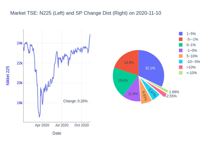
58.4% of stocks on TSE rose and 38.9% fell 51.7% of stocks on HKEx rose,36.1% fell 41.3% of stocks on NSE rose,56.5% fell 26.1% of stocks on SZE and SSE rose,71.9% stocks fell Asian Markets Summary Based on data of 2193 stocks traded on TSE 58.4% stocks rose,38.9% stocks fell 9.4% stocks jumped more than ..
This code is an example for calculating time difference in different units. It is a part of my one program. import pandas as pd DateOct02_2020=date(2020,10,2) # … data=pd.read_csv(file) data[‘Date’]=pd.to_datetime(data.Date) L=data.shape[0] for i in range(L): date1=data.loc[i,’Date’].date() ddt=DateOct02_2020-date1 print(int(ddt.total_seconds())) # in seconds print(int(ddt.total_seconds()/60)) # in minutes print(int(ddt.total_seconds()/60/60)) # in hours print(int(ddt.total_seconds()/60/60/24))..