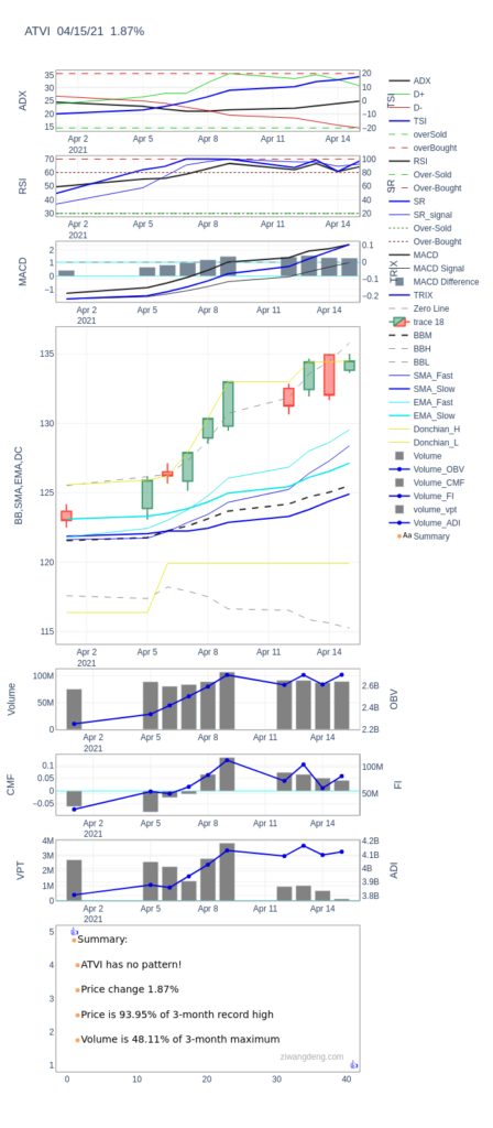
The following example shows you how to draw multiple subplots with different widths and heights. It also tells you the answers to some other questions.
- How to do technical analysis of a stock?
- How to draw double y-axis plot?
- How to set height of a subplot?
import numpy as np
import talib
import emoji
import pandas as pd
from datetime import datetime,date
from ta import add_all_ta_features
from ta.utils import dropna
import plotly.graph_objects as go
import chart_studio.plotly as py
from plotly.subplots import make_subplots
candleRank=pd.read_csv('CandleStick_rankings.csv')
candle_names = talib.get_function_groups()['Pattern Recognition']
candleRank=candleRank.set_index('Unnamed: 0')
#------------------------------------
Year=2020
Month=5
fnlist='nasdq100List.txt'
fns=pd.read_csv(fnlist)
path='nasdq100/'
#-------------------------------------
for fn0 in fns.symbles[:1]:
stockname=fn0.replace('.csv','')
fn=path + stockname + '.csv'
fn=fn.replace(' ','')
figfilename="images/nasdq100/" + stockname + '_Technical_Analysis.png'
figfilename=figfilename.replace(' ','')
df0=pd.read_csv(fn)
#! convert Date to datetime
df0['Date']=df0['Date'].astype('datetime64[ns]')
df0=df0.rename(columns={'Date':'date'})
#! drop nan data
df0 = dropna(df0)
df0 = add_all_ta_features(df0, open="Open", high="High", low="Low", close="Close", volume="Volume")
df=df0.iloc[-62:]
minVolume=df['Volume'].min()
maxVolume=df['Volume'].max()
minClose=df['Close'].min()
maxClose=df['Close'].max()
strdate=df["date"].dt.strftime("%m/%d/%y").iloc[-1]
tradingClosePCT=np.round((df0.Close.iloc[-1]/maxClose)*100,2)
tradingVolumePCT=np.round((df0.Volume.iloc[-1]/maxVolume)*100,2)
str4Volume="Volume is " + str(tradingVolumePCT) +'% of 3-month maximum'
if(df['Volume'].tail(1).values ==minVolume):
str4Volume='Trading volume hits 3-month record low.'
if(df['Volume'].tail(1).values ==maxVolume):
str4Volume='Trading volume hits 3-month record high.'
str4Close='Price is ' + str(tradingClosePCT) +'% of 3-month record high'
if(df.Close.tail(1).values==minClose):
str4Close='Close price dips to the 3-month record low.'
if(df.Close.tail(1).values==maxClose):
str4Close='Close price soars to the 3-month record high.'
ratePCT=np.round((df0.Close.iloc[-1]/df0.Close.iloc[-2]-1)*100,2)
strPriceChange='Price change ' + str(ratePCT) +'%'
if(ratePCT>5):
strPriceChange='Price soars ' + str(ratePCT) +'%'
if(ratePCT<-5):
strPriceChange='Price dips ' + str(ratePCT) +'%'
df1=df0.iloc[-5:]
op=df1['Open']
hi=df1['High']
lo=df1['Low']
cl=df1['Close']
pattern_columns=['Open_2','High_2','Low_2','Close_2','Open_1','High_1','Low_1','Close_1'] \
+ list(df.columns) + ['PatternName','Bull2Bear']
df_pattern=pd.DataFrame(columns=pattern_columns)
for candle in candle_names:
df[candle] = getattr(talib, candle)(op, hi, lo, cl)
df=df[candle_names].tail(1)
#print(df[candle_names])
df_candles=df[candle_names].sum(axis=1)
if(df_candles.values==0):
aboutThePatterns = stockname + " has no pattern!"
else:
for candle in candle_names:
if(df[candle].values==0):
df=df.drop(candle,axis=1)
aboutThePatterns=''
for col in df.columns:
if(df[col].values<0):
bull2bear=col + '_Bear'
else:
bull2bear=col+ '_Bull'
if (bull2bear in list(candleRank.index)):
strRank=str(candleRank.loc[bull2bear,'Rank'])
else:
strRank=''
aboutThePatterns = aboutThePatterns + \
"Pattern(s): " + \
bull2bear + ",Rank=" + strRank
aboutThePatterns=aboutThePatterns.replace(' ',' ').replace('CDL','')
s1='<img src="https://github.com/ziwangdeng/TechnicalAnalysis/blob/master/nasdq/'
s2=stockname + '_Technical_Analysis.png?raw=true"'
s2=s2.replace(' ','').replace('.TO','_TO')
s3=' alt="Technical_Analysis" width="100%" height="1600"><br>'
ss=s1 + s2 + s3
print(ss)
df=df0.iloc[-10:]
#! set subplot heights
fig = make_subplots(
rows=12, cols=1,
specs=[
[{"rowspan":1,"secondary_y": True}],
[{"rowspan":1,"secondary_y": True}],
[{"rowspan":1,"secondary_y": True}],
[{"rowspan":4,"secondary_y": False}],
[None],
[None],
[None],
[{"rowspan":1,"secondary_y": True}],
[{"rowspan":1,"secondary_y": True}],
[{"rowspan":1,"secondary_y": True}],
[{"rowspan":2,"secondary_y": False}],
[None],
])
# ADX
fig.add_trace(go.Scatter(x=df.date,
y=df.trend_adx,
mode='lines',
name="ADX",
line=dict(color='rgb(30,30,30)',
width=2)),row=1,col=1,secondary_y=False)
fig.add_trace(go.Scatter(x=df.date,
y=df.trend_adx_pos,
mode='lines',
name="D+",
line=dict(color='rgb(0,200,0)',
width=1)),row=1,col=1,secondary_y=False)
fig.add_trace(go.Scatter(x=df.date,
y=df.trend_adx_neg,
mode='lines',
name="D-",
line=dict(color='rgb(200,0,0)',
width=1)),row=1,col=1,secondary_y=False)
#TSI
#! double yaxes
fig.add_trace(go.Scatter(x=df.date,
y=df.momentum_tsi,
mode='lines',
name="TSI",
line=dict(color='rgb(0,0,230)',
width=2)),row=1,col=1,secondary_y=True)
x1=df.date.iloc[0]
x2=df.date.iloc[-1]
y1=-20
y2=20
fig.add_trace(go.Scatter(x=[x1,x2],
y=[y1,y1],
mode='lines',
name='overSold',
line=dict(color='rgb(0,200,0)',
width=1,dash='dash')),row=1,col=1,secondary_y=True)
fig.add_trace(go.Scatter(x=[x1,x2],
y=[y2,y2],
mode='lines',
name='overBought',
line=dict(color='rgb(200,0,0)',
width=1,dash='dash')),row=1,col=1,secondary_y=True)
#RSI
fig.add_trace(go.Scatter(x=df.date,
y=df.momentum_rsi,
mode='lines',
name="RSI",
line=dict(color='rgb(30,30,30)',
width=2)),row=2,col=1,secondary_y=False)
x1=df.date.iloc[0]
x2=df.date.iloc[-1]
y1=30
y2=70
fig.add_trace(go.Scatter(x=[x1,x2],
y=[y1,y1],
mode='lines',
name='Over-Sold',
line=dict(color='rgb(0,200,0)',
width=1,dash='dash')),row=2,col=1,secondary_y=False)
fig.add_trace(go.Scatter(x=[x1,x2],
y=[y2,y2],
mode='lines',
name='Over-Bought',
line=dict(color='rgb(200,0,0)',
width=1,dash='dash')),row=2,col=1,secondary_y=False)
# SR
fig.add_trace(go.Scatter(x=df.date,
y=df.momentum_stoch,
mode='lines',
name="SR",
line=dict(color='rgb(0,0,230)',
width=2)),row=2,col=1,secondary_y=True)
fig.add_trace(go.Scatter(x=df.date,
y=df.momentum_stoch_signal,
mode='lines',
name="SR_signal",
line=dict(color='rgb(0,0,230)',
width=1)),row=2,col=1,secondary_y=True)
x1=df.date.iloc[0]
x2=df.date.iloc[-1]
y1=20
y2=80
fig.add_trace(go.Scatter(x=[x1,x2],
y=[y1,y1],
mode='lines',
name='Over-Sold',
line=dict(color='rgb(0,100,0)',
width=1,dash='dot')),row=2,col=1,secondary_y=True)
fig.add_trace(go.Scatter(x=[x1,x2],
y=[y2,y2],
mode='lines',
name='Over-Bought',
line=dict(color='rgb(100,0,0)',
width=1,dash='dot')),row=2,col=1,secondary_y=True)
#MACD
fig.add_trace(go.Scatter(x=df['date'],
y=df.trend_macd,
mode='lines',
line=dict(color='rgb(30,30,30)',width=2), name="MACD"),row=3,col=1,secondary_y=False)
fig.add_trace(go.Scatter(x=df['date'],
y=df.trend_macd_signal,mode='lines',
line=dict(color='rgb(30,30,30)',width=1),
name="MACD Signal"),row=3,col=1,secondary_y=False)
fig.add_trace(go.Bar(x=df['date'],
y=df.trend_macd_diff,
base=0,
marker_color='lightslategrey',
name="MACD Difference"),row=3,col=1,secondary_y=False)
#TRIX
fig.add_trace(go.Scatter(x=df.date,
y=df.trend_trix,
mode='lines',
name="TRIX",
line=dict(color='rgb(0,0,230)',
width=2)),row=3,col=1,secondary_y=True)
x1=df.date.iloc[0]
x2=df.date.iloc[-1]
y1=0
y2=0
fig.add_trace(go.Scatter(x=[x1,x2],
y=[y1,y1],
mode='lines',
name='Zero Line',
line=dict(color='rgb(130,130,130)',
width=1,dash='dash')),row=3,col=1,secondary_y=True)
# bollinger band
fig.add_trace(go.Candlestick(x=df['date'],
open=df['Open'],
high=df['High'],
low=df['Low'],
close=df['Close']
),row=4,col=1)
fig.add_trace(go.Scatter(x=df.date,
y=df.volatility_bbm,
mode='lines',
name="BBM",
line=dict(color='rgb(30,30,30)', width=2, dash='dash')),row=4,col=1)
fig.add_trace(go.Scatter(x=df.date,
y=df.volatility_bbh,
mode='lines', name="BBH",
line=dict(color='rgb(130,130,130)', width=1, dash='dash')),row=4,col=1)
fig.add_trace(go.Scatter(x=df.date,
y=df.volatility_bbl,
mode='lines',
name="BBL",
line=dict(color='rgb(130,130,130)', width=1, dash='dash')),row=4,col=1)
fig.add_trace(go.Scatter(x=df.date,
y=df.trend_sma_fast,
mode='lines',
name="SMA_Fast",
line=dict(color='rgb(0,0,230)', width=1)),row=4,col=1)
fig.add_trace(go.Scatter(x=df.date,
y=df.trend_sma_slow,
mode='lines',
name="SMA_Slow",
line=dict(color='rgb(0,0,230)', width=2)),row=4,col=1)
fig.add_trace(go.Scatter(x=df.date,
y=df.trend_ema_fast,
mode='lines',
name="EMA_Fast",
line=dict(color='rgb(0,230,230)', width=1)),row=4,col=1)
fig.add_trace(go.Scatter(x=df.date,
y=df.trend_ema_slow,
mode='lines',
name="EMA_Slow",
line=dict(color='rgb(0,230,230)', width=2)),row=4,col=1)
fig.add_trace(go.Scatter(x=df.date,
y=df.volatility_dch,
mode='lines',
name="Donchian_H",
line=dict(color='rgb(230,230,0)', width=1)),row=4,col=1)
fig.add_trace(go.Scatter(x=df.date,
y=df.volatility_dcl,
mode='lines',
name="Donchian_L",
line=dict(color='rgb(230,230,0)', width=1)),row=4,col=1)
# Volume
fig.add_trace(go.Bar(x=df.date,
y=df.Volume,
base=0,
name="Volume",
marker_color='rgb(130,130,130)'),row=8,col=1,secondary_y=False)
# Volume OBV
fig.add_trace(go.Scatter(x=df.date,
y=df.volume_obv,
name="Volume_OBV",
line=dict(color='rgb(0, 0, 230)',
width=2)),row=8,col=1,secondary_y=True)
# Chaikin Money Flow (CMF)
basevalue=df.volume_cmf.min
fig.add_trace(go.Bar(x=df.date,
y=df.volume_cmf,
name="Volume_CMF",
marker_color='rgb(130,130,130)'),row=9,col=1,secondary_y=False)
# FI
# basevalue=df.volume_cmf.min
fig.add_trace(go.Scatter(x=df.date,
y=df.volume_fi,
name="Volume_FI",
line=dict(color='rgb(0, 0, 230)',
width=2)),row=9,col=1,secondary_y=True)
# Volume-price Trend (VPT)
fig.add_trace(go.Bar(x=df.date,
y=df.volume_vpt,
base=0,
name="volume_vpt",
marker_color='rgb(130,130,130)'),row=10,col=1,secondary_y=False)
# ADI
fig.add_trace(go.Scatter(x=df.date,
y=df.volume_adi,
name="Volume_ADI",
line=dict(color='rgb(0, 0, 230)',
width=2)),row=10,col=1,secondary_y=True)
fig.add_annotation(
x=1,
y=5,
ax=1,ay=0,
font=dict(color='blue'),
text=emoji.emojize(':thumbs_up:'),row=11,col=1)
fig.add_annotation(
x=41,
y=1,
ax=1,ay=0,
font=dict(color='blue'),
text=emoji.emojize(':thumbs_up:'),row=11,col=1)
fig.add_trace(go.Scatter(
x=[1,1.5,1.5,1.5,1.5,1.5],
y=[4.75,4.00,3.25,2.5,1.75],
name="Summary",
mode='markers+text',
text=['Summary:',aboutThePatterns,strPriceChange,str4Close,str4Volume],
textposition='middle right',
textfont=dict(family='sans serif',
size=14,
color='black')),row=11,col=1)
fig.add_annotation( x=35,
y=1.25,
ax=1,ay=0,font=dict(color='#aaaaaa'),
text="ziwangdeng.com",row=11,col=1)
fig.update_yaxes(title_text="ADX", row=1, col=1,secondary_y=False,
showline=True,linecolor='#888888', mirror=True,
showgrid=True, gridwidth=1, gridcolor='#eeeeee')
fig.update_yaxes(title_text="TSI", row=1, col=1,secondary_y=True,
showline=True,linecolor='#888888', mirror=True,
showgrid=True, gridwidth=1, gridcolor='#eeeeee')
fig.update_xaxes(row=1,col=1,
showline=True,linecolor='#888888', mirror=True,
showgrid=True, gridwidth=1, gridcolor='#eeeeee')
fig.update_yaxes(title_text="RSI", row=2, col=1,secondary_y=False,
showline=True,linecolor='#888888', mirror=True,
showgrid=True, gridwidth=1, gridcolor='#eeeeee')
fig.update_yaxes(title_text="SR", row=2, col=1,secondary_y=True,
showline=True,linecolor='#888888', mirror=True,
zerolinewidth=1, zerolinecolor='#00ffff',
showgrid=True, gridwidth=1, gridcolor='#eeeeee')
fig.update_xaxes(row=2,col=1,
showline=True,linecolor='#888888', mirror=True,
showgrid=True, gridwidth=1, gridcolor='#eeeeee')
fig.update_yaxes(title_text="MACD", row=3, col=1,secondary_y=False,
showline=True,linecolor='#888888', mirror=True,
zerolinewidth=1, zerolinecolor='#00ffff',
showgrid=True, gridwidth=1, gridcolor='#eeeeee')
fig.update_yaxes(title_text="TRIX", row=3, col=1,secondary_y=True,
showline=True,linecolor='#888888', mirror=True,
zerolinewidth=1, zerolinecolor='#00ffff',
showgrid=True, gridwidth=1, gridcolor='#eeeeee')
fig.update_xaxes(row=3,col=1,
showline=True,linecolor='#888888', mirror=True,
showgrid=True, gridwidth=1, gridcolor='#eeeeee')
fig.update_yaxes(title_text="BB,SMA,EMA,DC", row=4, col=1,secondary_y=False,
showline=True,linecolor='#888888', mirror=True,
showgrid=True, gridwidth=1, gridcolor='#eeeeee')
fig.update_xaxes(row=4,col=1,
showline=True,linecolor='#888888', mirror=True,
showgrid=True, gridwidth=1, gridcolor='#eeeeee')
fig.update_yaxes(title_text="Volume", row=8, col=1,secondary_y=False,
showline=True,linecolor='#888888', mirror=True,
showgrid=True, gridwidth=1, gridcolor='#eeeeee')
fig.update_yaxes(title_text="OBV", row=8, col=1,secondary_y=True)
fig.update_xaxes(row=8,col=1,
showline=True,linecolor='#888888', mirror=True,
showgrid=True, gridwidth=1, gridcolor='#eeeeee')
fig.update_yaxes(title_text="CMF", row=9, col=1,secondary_y=False,
showline=True,linecolor='#888888', mirror=True,
zerolinewidth=1, zerolinecolor='#00ffff',
showgrid=True, gridwidth=1, gridcolor='#eeeeee')
fig.update_yaxes(title_text="FI", row=9, col=1,secondary_y=True,
showline=True,linecolor='#888888', mirror=True,
showgrid=True, gridwidth=1, gridcolor='#eeeeee')
fig.update_xaxes(row=9,col=1,
showline=True,linecolor='#888888', mirror=True,
showgrid=True, gridwidth=1, gridcolor='#eeeeee')
fig.update_yaxes(title_text="VPT", row=10, col=1,secondary_y=False,
showline=True,linecolor='#888888', mirror=True,
zerolinewidth=1, zerolinecolor='#00ffff',
showgrid=True, gridwidth=1, gridcolor='#eeeeee')
fig.update_yaxes(title_text="ADI", row=10, col=1,secondary_y=True,
showline=True,linecolor='#888888', mirror=True,
showgrid=True, gridwidth=1, gridcolor='#eeeeee')
fig.update_xaxes(row=10,col=1,
showline=True,linecolor='#888888', mirror=True,
showgrid=True, gridwidth=1, gridcolor='#eeeeee')
fig.update_yaxes(row=11, col=1,showline=True,linecolor='#888888',
mirror=True,showgrid=False,zeroline=False)
fig.update_xaxes(row=11,col=1,showline=True,linecolor='#888888',
mirror=True,showgrid=False,zeroline=False)
fig.update_layout(height=1600,
title_text=stockname + ' ' + strdate + ' ' + str(ratePCT)+'%',
xaxis4 = {"rangeslider": {"visible": False}},
plot_bgcolor='rgb(255,255,255)'
)
fig.update_annotations(dict(showarrow=False),row=11,col=1)
fig.show()
fig.write_image(figfilename)